Weighted Variance

I had to review some basic statistics, so I figured I'd post a quick summary.  I tend to forget how to treat error when averaging, so this is a good reminder.

If we have a series of measurements  with variances , we might like to average them.  But, how should we weight them?

The standard way to weight such points is by inverse variance, which is the part I tend to forget:


We recall that a weighted average is:



The weighted variance of these points is much as you'd expect, but with a correction for the effective number of points.  That's the tricky part.



where the effective number of points is



Source: Lyons' Statistics for Nuclear and Particle Physicists

Charged Pion Branching Ratio: Part I

Inherent symmetries in nature lead to conservation laws (perhaps someone will make a post about Noether's Theorem). When we think about the stability of a sub-atomic particle we must think in these terms. Take for example the charged pion, in free space at the tree level. The particle* has mass and charge. (Don't forget to boost into the pion's rest frame) There are no lighter charged hadrons therefore the final state must include a charged lepton of less mass (ie an electron or muon). Our situation looks as follows

Now we invoke conservation of lepton number and conclude that we cannot make the lepton without an associated anti-lepton; charge conservation rules out all particles save neutrinos. So now we have

This situation is the end of the story for the vast majority of pion decays (99,999,999/100,000,000 times in fact). However we can sneak in another particle! The neutral pion is less massive than the charged pion by more than the mass of the electron so we can add a pi-zero to the electron channel (beta decay). We have now arrived at the complete picture.

The next step is to calculate the different decay rates for the various processes and that is a topic for part II!

* I'm playing fast and loose with what is a particle and what is an anti-particle, deal with it.

Mandelstam Variables

Two particle into two particle scattering is a common topic in the field of particle physics and is studied so often that special notation has been developed to facilitate discussion of such processes. The convention uses the "so-called" Mandelstam variables (s,t,u) where (p_i) represents the momentum of the four particles ():

These variables completely describe the momentum space of the problem in a Lorentz invariant way. One of the useful properties of this choice of variables is the fact that:

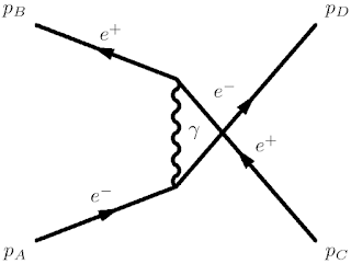
Furthermore we can elucidate these conditions by drawing the corresponding Feynman diagrams for each process.

s-channel

t-channel

u-channel

Gnuplot Fitting

If you aren't using gnuplot, you should check it out.  For those that do, I just figured out a fun tidbit on how to print fit errors that I couldn't find on the Intarwebs for the life of me.

The "fit" command in gnuplot works much like the "plot" command; you give it a data file and a "using" specification, and also the function you want to fit with and its parameters like so:

f(x) = a*x + b
a = -0.01
b = 0
fit f(x) 'somefile.txt' using 1:2:3 via a,b

You do need to give a first guess for parameters, as you see above.  The "using" specification here tells it to use the first column for x, second for y and the third for error in y (which you want to include if you can).  I've had plenty of trouble in the past getting a fit to converge, but generally you need to keep playing with your initial parameters and things will work out.  Once the fit is done you get something like this:

After 4 iterations the fit converged.
final sum of squares of residuals : 8.19305
rel. change during last iteration : -6.6513e-10


degrees of freedom    (FIT_NDF)                        : 9
rms of residuals      (FIT_STDFIT) = sqrt(WSSR/ndf)    : 0.954117
variance of residuals (reduced chisquare) = WSSR/ndf   : 0.910339


Final set of parameters            Asymptotic Standard Error
=======================            ==========================


a               = -0.00123217      +/- 0.0002571    (20.87%)
b               = 0.0347759        +/- 0.001622     (4.665%)


correlation matrix of the fit parameters:
               a      b      
a               1.000 
b              -0.872  1.000 

Huzzah!  You get your final fit parameters with error; you get degrees of freedom and stdfit and chisquare.  This is fun and all, but how to I put that in my plot?  First, you can get at some environment variables to use in your gnuplot script, like "FIT_WSSR" and "FIT_STDFIT."  As far as the final parameters and errors, here's the best way I've found to put them on your plot:

set fit errorvariables

fit f(x) 'group_asym_out.txt' index 1 u 1:2:3 via a,b 

set label sprintf("a = %2.6f +- %2.6f",a,a_err) at graph 0.7,0.15

set label sprintf("b = %2.6f +- %2.6f",b,b_err) at graph 0.7,0.1

plot 'somefile.txt' u 1:2:3 w yerr, f(x) title 'f(x)=a*x+b'

Here I've put the tricky part in bold.  We have to set labels on the graph somewhere; mercifully we can use the "graph" coordinates instead of the coordinates of the plot itself, so that top right is graph (1,1) and bottom left is graph (0,0).  Now we access our parameters "a" and "b" using "sprintf" in the label.

To get the errors on these parameters, we need to include "set fit errorvariables" which enables the error variables "_err," for example "a_err" and "b_err."  The graph still needs some stylistic attention, but at this point it looks this:

Sources: Janert's Gnuplot in Action

Čerenkov Radiation Application

Last week I gave a quick run-down of the justification of Cherenkov radiation from classical electrodynamics.  In practice, this effect is the centerpiece of many experiments, and I'll run through how and what we need to know in this post.

We recall the velocity of the charge particle must exceed the phase velocity of the E&M field to emit Cherenkov radiation, or with index of refraction n:



Cherenkov radiation comes in the form of an electromagnetic shock wave, a conical wavefront formed following the particle, emitted at angle:



Since we'd like to pick up this radiation in photomultiplier tubes to observe the effect and therewith the incident charge particle, it's good to know how many photons to expect.  Following the math of the last post on Cherenkov radiation (or just following along in Jackson), we take the energy differential over frequency and divide by de Broglie's h bar omega and then by L we get the number of photons per unit length:



Cherenkov radiation contributes to the mechanism of several types of particle detectors, including electromagnetic calorimeters and non-scintillating hodoscopes; there are two types of detectors specifically designed to directly take advantage of the Cherenkov radition emitted by high energy charge particles: threshold Cherenkov detectors and differential Cherenkov detectors.

In the threshold Cherenkov detector, the medium in the tank is chosen carefully for a refractive index that indicates the passage of charge particles that exceed a given velocity threshold.  Usually this is done with a gas such as hydrogen, nitrogen or carbon dioxide, and further control of the refractive index comes through the pressure of the gas in the tank.

The differential Cherenkov detector allows the measurement of a particle's velocity while rejecting particles outside a given mass range.  This is accomplished by accepting a small annulus around the track of incident particles at some angle theta.  This corresponds, at a given refractive index, to a velocity resolution:



The minimum velocity resolution is often constrained by the minimum angular resolution, which tends to be limited by dispersion in the slit.

Sources:  Leo's Techniques and Fernow's Intro to Experimental Particle Physics

Radiation Sources You Should Know

When working with particle detectors it is important to be able to confirm they are functioning properly. Often this process involves using calibrated radioactive sources. Care should be taken to use a source which produces radiation similar to what the detector is designed to measure. I was recently informed by Andries that (begin paraphrase) Someone at your level should really have memorized all the useful sources (end paraphrase). Once again the great work of Science-Nonfiction by Leo comes to the rescue. Here is a summary of the common sources particle physicist use (from Leo).

You know nothing

It is common for physics grad students to remember the angular momentum operator . Many will even remember that it commutes with and we can therefore form a set of simultaneous eigenfunctions to describe a particle in angular momentum space. Some may even recall that the standard conventions yield the following eigenequations.

But do you know how to demonstrate that and are the eigenvalues for and ?

for Stache: